BlobTracking

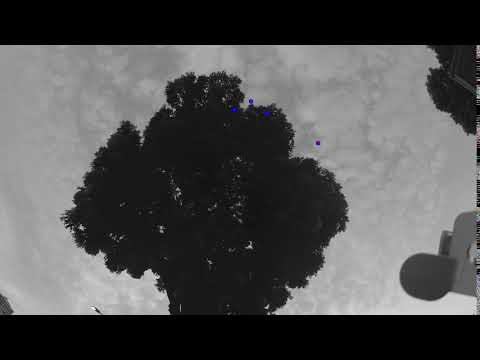
Detect and track blobs (like birds or bugs) moving around in an image. Blobs are detected using simple Laplacian-of-Gaussian filtering (from Images.jl) and tracked using a Kalman filter from LowLevelParticleFilters.jl.

This package contains some facilities for the aforementioned detection and tracking, as well as some utilities for background removal etc.

In the example below, we are tracking birds that fly around a tree.

using BlobTracking, Images, VideoIO
path = "/home/fredrikb/Video/2_small.MP4"
io   = VideoIO.open(path)
vid  = VideoIO.openvideo(io)
img  = first(vid)

this package implements an iterator for VideoIO videos. It only iterates black and white images, even if the original video is in color.

We create a background image to subtract from each image

medbg = MedianBackground(Float32.(img), 4) # A buffer of 4 frames
foreach(1:4) do i # Populate the buffer
    update!(medbg,Float32.(first(vid)))
end
bg = background(medbg)

If you want to detect birds (blobs) in the entire image, you can skip this step.

A mask is a binary image that is true where you want to be able to detect blobs and false where you want to ignore.

mask = (bg .> 0.4) |> reduce(∘, fill(erode, 30)) |> reduce(∘, fill(dilate, 20))
mask[:,1190:end] .= 0
mask[end-50:end,:] .= 0

For the tracking to work well, it's important that we feed the tracker nice and clean images. An example of a pre-processing function looks like this, it takes a storage array you can operate on in-place and the image to pre-process.

function preprocessor(storage, img)
    storage .= Float32.(img)
    update!(medbg, storage) # update the background model
    storage .= Float32.(abs.(storage .- background(medbg)) .> 0.4) # You can save some computation by not calculating a new background image every sample
end

Notice how the tree contours are still present in this image? This is okay since that is behind the mask we created above. The mask was created by dilating the tree slightly so that the mask covers slightly more than the tree. However, in this image you can also see two small spots to the right of the tree, representing birds.

We now create the BlobTracker and run the tracking. If we don't know an appropriate value for the sizes vector that determines the size scales of the blobs, we may call the function tune_sizes to get a small GUI with a slider to help us out (works in Juno and IJulia). The length of sizes has a large impact on the time it takes to process each frame since the majority of the processing time is taken up by the blob detection.

bt = BlobTracker(3:3, #sizes 
                2.0, # σw Dynamics noise std.
                10.0,  # σe Measurement noise std. (pixels)
                mask=mask,
                preprocessor = preprocessor,
                amplitude_th = 0.05,
                correspondence = HungarianCorrespondence(p=1.0, dist_th=2), # dist_th is the number of sigmas away from a predicted location a measurement is accepted.
)
tune_sizes(bt, img)

result = track_blobs(bt, vid,
                         display = Base.display, # use nothing to omit displaying.
                         recorder = Recorder()) # records result to video on disk

To display images in a standalone window with okay performance, consider

using ImageView
c = imshow(img)
displayfun = img -> imshow!(c["gui"]["canvas"],img);
track_blobs(...; display = displayfun)

Blobs are shown in blue, newly spawned blobs are show in green and measurements are shown in red.If everything is working well, most blue dots should have a red dot inside or very nearby. If the blue blobs are lagging behind the red dots, the filter needs tuning by either decreasing the measurement variance or increasing the dynamics variance. If blue dots shoot off rapidly whenever measurements are lost, the dynamics variance should be decreased.

If you do not want to run the tracking and instead only collect all coordinates of detected blobs, you may call

coords = get_coordiantes(bt, vid)

you can then later call the tracking function like result = track_blobs(bt,coords), but if invoked like this, you do not have the option to display or record images.

traces = trace(result, minlife=5) # Filter minimum lifetime of 5
measurement_traces = tracem(result, minlife=5)
drawimg = RGB.(img)
draw!(drawimg, traces, c=RGB(0,0,0.5))
draw!(drawimg, measurement_traces, c=RGB(0.5,0,0))

In the image, green dots represent spawning positions and red dots the last obtained measurement for a blob in case of the red measurement traces, and the point at which the blob was killed in case of the blue location traces.

Below is a youtube video showing how it looks

Most functions have docstrings. Docstrings of types hint at what functions you can call on instances of the type. The types present in this package are

• Blob represents a Blob, contains traces of locations and measurements as well as the Kalman filter
• BlobTracker contains parameters for the tracking and correspondence matching
• KalmanParams stores the variance parameters for the KalmanFilter.
• AbstractCorrespondence
  • HungarianCorrespondence matches blobs to measurements using the Hungarian algorithm
  • NearestNeighborCorrespondence matches blobs to the nearest measurement
  • MCCorrespondence uses Monte Carlo integration over the filtering distribution of the blobs and matches blobs to measurements several times using the chosen inner AbstractCorrespondence.
• TrackingResult contains lists of dead and alive blobs
• Trace is a list of coordinates
• Recorder records movies and saves them on disk
• FrameBuffer stores frames for temporal processing
• BackgroundExtractor
  • MedianBackground models the background of an image
  • DiffBackground models the background of an image
• Workspace is used internally