NTFk is a module of the SmartTensors ML framework (smarttensors.com).
NTFk performs a novel unsupervised Machine Learning (ML) method based on Tensor Decomposition (Factorization) coupled with constraints (sparsity, nonnegativity, physical, mathematical).
NTFk methodology allows for automatic identification of the optimal number of features (signals) present in multi-dimensional data arrays (tensors). The number of features (tensor rank / multi-rank) along different dimensions can be estimated jointly and independently.
SmartTensors can be applied to perform various types of analyses of multi-dimensional data:
- Feature extraction (FE)
- Blind source separation (BSS)
- Detection of disruptions/anomalies
- Image recognition
- Text mining
- Data classification
- Separation (deconstruction) of co-occurring (physics) processes
- Discovery of unknown dependencies and phenomena
- Development of reduced-order/surrogate models
- Identification of dependencies between model inputs and outputs
- Guiding the development of physics models representing the ML-analyzed data
- Blind predictions
- Optimization of data acquisition (optimal experimental design)
- Labeling of datasets for supervised ML analyses
NTFk provides high-performance computing capabilities to solve problems with Shared and Distributed Arrays in parallel. The parallelization allows for the utilization of multi-core / multi-processor environments. GPU and TPU accelerations are available through existing Julia packages.
NTFk can be employed to perform tensor decomposition using CP (Candecomp/Parafac) and Tucker methods.
NTFk provides options to access existing tensor decomposition methods available in MATLAB (MATLAB installation required):
- Tamara Kolda's TensorToolbox
- Ivan Oseledets' TT-Toolbox
- Wotao Yin's BCU
- TensorLab
NTFk provides also an interface to Jean Kossaifi's Python TensorLy.
NTFk can perform high-performance computing tensor decomposition analyses using TensorFlow, PyTorch, and MXNET.
NTFk methodology and applications are discussed in the papers and presentations listed below.
Tensor network decompositions can be performed using SmartTensors' NTNk package.
Matrix factorization can be performed using SmartTensors' NMFk package.
SmartTensors and NTFk were recently awarded:
- 2021 R&D100 Award: Information Technologies (IT)
- 2021 R&D100 Bronze Medal: Market Disruptor in Services
After starting Julia, execute:
import Pkg
Pkg.add("NTFk")
to access the latest released version. To utilize the latest updates (commits), use:
import Pkg
Pkg.add(Pkg.PackageSpec(name="NTFk", rev="master"))docker run --interactive --tty montyvesselinov/tensorsThe docker image provides access to all SmartTensors packages (smarttensors.github.io).
import Pkg
Pkg.test("NTFk")NTFk performs a novel unsupervised Machine Learning (ML) method based on Tensor Decomposition coupled with sparsity and nonnegativity constraints.
NTFk has been applied to extract the temporal and spatial footprints of the features in multi-dimensional datasets in the form of multi-way arrays or tensors.
NTFk executes the decomposition (factorization) of a given tensor by minimization of the Frobenius norm:
where:
is the dimensionality of the tensor
is a "mixing" core tensor
are "feature” factors (in the form of vectors or matrices)
is a tensor product applied to fold-in factors
in each of the tensor dimensions
The product is an estimate of
(
).
The reconstruction error is expected to be random uncorrelated noise.
is a
-dimensional tensor with a size and a rank lower than the size and the rank of
.
The size of tensor
defines the number of extracted features (signals) in each of the tensor dimensions.
The factor matrices represent the extracted features (signals) in each of the tensor dimensions.
The number of matrix columns equals the number of features in the respective tensor dimensions (if there is only 1 column, the particular factor is a vector).
The number of matrix rows in each factor (matrix)
equals the size of tensor X in the respective dimensions.
The elements of tensor define how the features along each dimension (
) are mixed to represent the original tensor
.
NTFk can perform Tensor Decomposition using Candecomp/Parafac (CP) or Tucker decomposition models.
Some of the decomposition models can theoretically lead to unique solutions under specific, albeit rarely satisfied, noiseless conditions.
When these conditions are not satisfied, additional minimization constraints can assist the factorization.
A popular approach is to add sparsity and nonnegative constraints.
Sparsity constraints on the elements of G reduce the number of features and their mixing (by having as many zero entries as possible).
Nonnegativity enforces parts-based representation of the original data, which also allows the Tensor Decomposition results for and
to be easily interrelated Cichocki et al, 2009.
A simple problem demonstrating NTFk can be executed as follows. First, generate a random Tucker tensor:
import NTFk

csize = (2, 3, 4)
tsize = (5, 10, 15)
tucker_orig = NTFk.rand_tucker(csize, tsize; factors_nonneg=true, core_nonneg=true)
After that, we can compose a tensor-based on this Tucker decomposition:
import TensorDecompositions

T_orig = TensorDecompositions.compose(tucker_orig)
T_orig .*= 1000
Applying NTFk, we can find the unknown core size of the tensor using the tensor by itself as an input only. To do this, we explore a series of core sizes and identify the optimal one:
sizes = [csize, (1,3,4), (3,3,4), (2,2,4), (2,4,4), (2,3,3), (2,3,5)]
tucker_estimated, csize_estimated = NTFk.analysis(T_orig, sizes, 3; eigmethod=[false,false,false], progressbar=false, tol=1e-16, max_iter=100000, lambda=0.);
NTFk execution will produce something like this:
[ Info: Decompositions (clustering dimension: 1)
1 - (2, 3, 4): residual 5.46581369842339e-5 worst tensor correlations [0.999999907810158, 0.9999997403618763, 0.9999995616299466] rank (2, 3, 4) silhouette 0.9999999999999997
2 - (1, 3, 4): residual 0.035325052042119755 worst tensor correlations [0.9634250567157897, 0.9842244237924007, 0.9254792458530211] rank (1, 3, 3) silhouette 1.0
3 - (3, 3, 4): residual 0.00016980024483822563 worst tensor correlations [0.9999982865486768, 0.9999923375643894, 0.9999915188040427] rank (3, 3, 4) silhouette 0.9404124172744835
4 - (2, 2, 4): residual 0.008914390317042747 worst tensor correlations [0.99782068249921, 0.9954301522732436, 0.9849956624171726] rank (2, 2, 4) silhouette 1.0
5 - (2, 4, 4): residual 0.00016061795564929862 worst tensor correlations [0.9999980289931861, 0.999996821183636, 0.9999940994076768] rank (2, 4, 4) silhouette 0.9996306553034816
6 - (2, 3, 3): residual 0.004136013571334162 worst tensor correlations [0.999947037606024, 0.9989851398124378, 0.9974723120905729] rank (2, 3, 3) silhouette 0.9999999999999999
7 - (2, 3, 5): residual 7.773676978117656e-5 worst tensor correlations [0.9999997131266367, 0.999999385995213, 0.9999988336042696] rank (2, 3, 5) silhouette 0.9999359399113312
[ Info: Estimated true core size based on the reconstruction: (2, 3, 4)
The final NTFk result is the estimated core size (2,3,4), which, as expected, matches the original unknown core size.
NTFk also produces a Tucker deconstruction of this tensor with core size (2,3,4), which is stored as tucker_estimated[ibest]
A series of Jupyter notebooks demonstrating NMFk have been developed:
The notebooks can also be accessed using:
NTFk.notebooks()NTFk has been applied in a wide range of real-world applications. The analyzed datasets include model outputs, laboratory experimental data, and field tests:
- Climate data and simulations
- Watershed data and simulations
- Aquifer simulations
- Surface-water and Groundwater analyses
- Material characterization
- Reactive mixing
- Molecular dynamics
- Contaminant transport
- Induced seismicity
- Phase separation of co-polymers
- Oil / Gas extraction from unconventional reservoirs
- Geothermal exploration and production
- Geologic carbon storage
- Wildfires
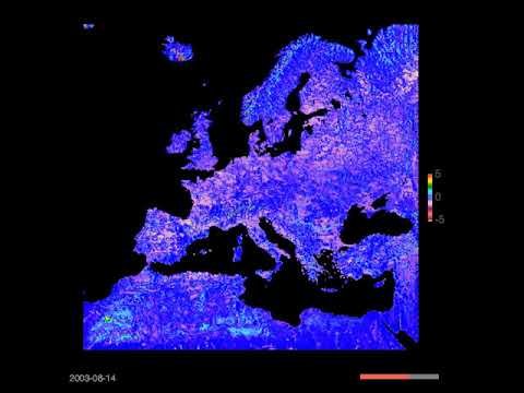
- Europe Climate Model: Water table fluctuations in 2003
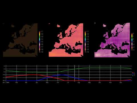
- Europe Climate Model: Deconstruction of water table fluctuations in 2003
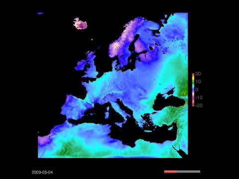
- Europe Climate Model: Air temperature fluctuations in 2003
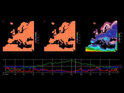
- Europe Climate Model: Deconstruction of Air temperature fluctuations in 2003
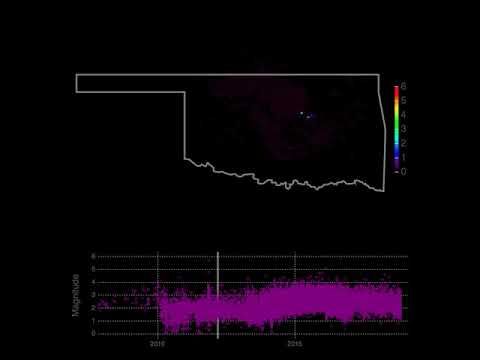
- Oklahoma seismic events
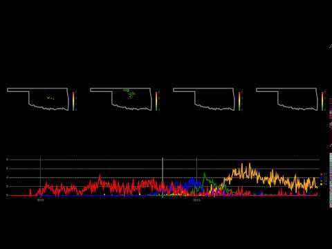
- Deconstruction of Oklahoma seismic events
- Deconstruction of Oklahoma seismic events
Videos are available on YouTube
- Vesselinov, V.V., Mudunuru, M., Karra, S., O'Malley, D., Alexandrov, B.S., Unsupervised Machine Learning Based on Non-Negative Tensor Factorization for Analyzing Reactive-Mixing, Journal of Computational Physics, 2018 (in review). PDF
- Vesselinov, V.V., Alexandrov, B.S., O'Malley, D., Nonnegative Tensor Factorization for Contaminant Source Identification, Journal of Contaminant Hydrology, 10.1016/j.jconhyd.2018.11.010, 2018. PDF
Research papers are also available at Google Scholar, ResearchGate and Academia.edu
- Vesselinov, V.V., Novel Machine Learning Methods for Extraction of Features Characterizing Datasets and Models, AGU Fall meeting, Washington D.C., 2018. PDF
- Vesselinov, V.V., Novel Machine Learning Methods for Extraction of Features Characterizing Complex Datasets and Models, Recent Advances in Machine Learning and Computational Methods for Geoscience, Institute for Mathematics and its Applications, University of Minnesota, 2018. PDF
Presentations are also available at slideshare.net, ResearchGate and Academia.edu
For more information, visit monty.gitlab.io, http://smarttensors.com [smarttensors.github.io],(https://smarttensors.github.io), and tensors.lanl.gov.


