InteractiveViz.jl

Interactive visualization tools for Julia

Julia already has a rich set of plotting tools in the form of the Plots and Makie ecosystems, and various backends for these. So why another plotting package?

InteractiveViz is not a replacement for Plots or Makie, but rather a graphics pipeline system developed on top of Makie. It has a few objectives:

• To provide a simple API to visualize large or possibly infinite datasets (tens of millions of data points) easily.
• To enable interactivity, and be responsive even with large amounts of data.
• To render perceptually accurate summaries at large scale, allowing drill down to individual data points.
• To allow generation of data points on demand through a graphics pipeline, requiring computation only at a level of detail appropriate for display at the viewing resolution. Additional data points can be generated on demand when zooming or panning.

This package was partly inspired by the excellent Datashader package available in the Python ecosystem.

This package does not aim to provide comprehensive production quality plotting. It is aimed at interactive exploration of large datasets.

Install InteractiveViz.jl with one of the Makie backends that support interactivity (GLMakie or WebGLMakie).

julia>]
pkg> add InteractiveViz GLMakie

If more than one Makie backend is available, switch between them in the usual way.

using GLMakie
GLMakie.activate!()

using WGLMakie
WGLMakie.activate!()

NOTE: InteractiveViz API and internals changed in v0.4. If you're familiar with the older API, do read through the documentation again. The functionality has not changed much, but the v0.4 uses the new Makie layout functionality and has improved its internal design to provide a more flexible data source API.

Let's start off visualizing a simple function of one variable:

julia> using InteractiveViz, GLMakie
julia> ilines(sin, 0, 100)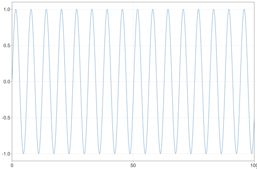

This displays the sin() function with the initial view set to the x-range of 0 to 100. You can however, pan and zoom (as you would do with a normal GLMakie window) beyond this range.

Let's next try plotting 2 timeseries, each with 10 million points:

julia> ilines(5*sin.(0.02π .* (1:10000000)))
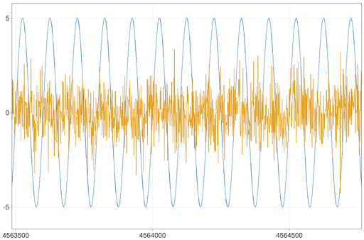
julia> ilines!(randn(10000000))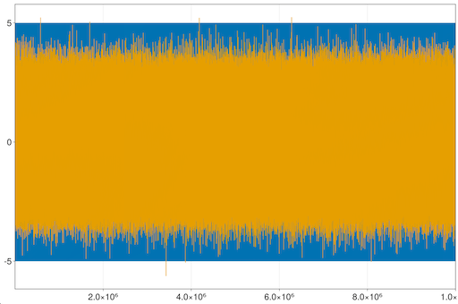

You can zoom and pan to see details:

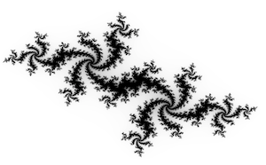
Next, let us visualize the famous Mandelbrot set:

julia> using InteractiveViz.Demo
julia> iheatmap(mandelbrot, -2, 0.66, -1, 1)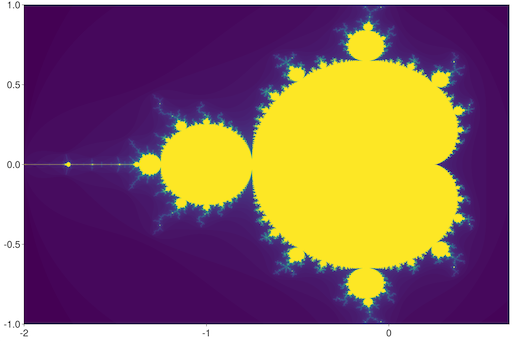

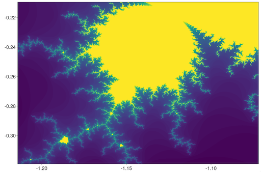
Try zooming in to a tiny part of the image, and see the fractal nature of the image render itself dynamically at full resolution!

And how can we forget the Julia set?

julia> iheatmap(julia, -2, 2, -1.75, 1.75; colormap=:magma)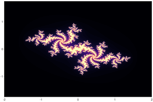

You could of course plot a large heatmap stored in a matrix as well:

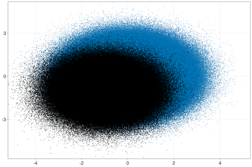
julia> iheatmap(range(0, 10; length=1000), range(0, 1; length=10000), randn(1000,10000))

Finally, let's try a scatter plot with ten million points:

julia> iscatter(randn(10_000_000), randn(10_000_000); markersize=3)

and add on another hundred thousand ones:

julia> iscatter!(randn(1_000_000) .- 1, randn(1_000_000) .- 1; color=:black, markersize=4)

Try zooming into this plot and see that it remains responsive as you zoom down to each individual point, or zoom out to get a birds-eye view!

While we haven't documented all the keyword options here, you'll find that all of the plot attributes for Makie work as options in InteractiveViz.

All of Makie's layout API also works as expected:

julia> using GLMakie
julia> f = Figure()
julia> p1 = iheatmap(f[1,1], julia, -2, 2, -1.75, 1.75; colormap=:magma)
julia> p2 = iheatmap(f[2,1], mandelbrot, -2, 0.66, -1, 1)
julia> Colorbar(f[1,2], p1.plot)
julia> Colorbar(f[2,2], p2.plot)
julia> p3 = ilines(f[1,3], sin, 0, 100; axis=(; limits=(0, 100, -1.5, 1.5)))
julia> p4 = ilines(f[2,3], range(0, 100; length=10000), randn(10000))
julia> linkxaxes!(p3.axis, p4.axis)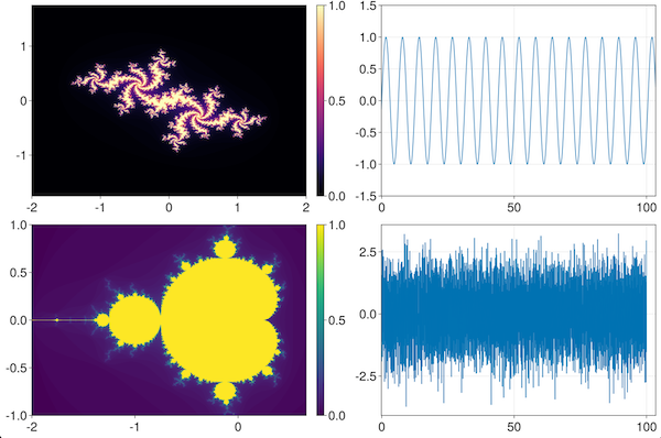

All InteractiveViz data sources are subtypes of the abstract DataSource type. Currently, three abstract subtypes of data sources are defined:

• Continuous1D for continuous one-dimensional data (e.g. time series),
• Continuous2D for continuous two-dimensional data (e.g. 2D topography heatmaps), and
• PointSet for discrete points (e.g. scatter plots).

The API to implement for each data source simply consists of two methods:

sample(data::DataSource, xrange::StepRangeLen, yrange::StepRangeLen)
limits(data::DataSource)

sample() samples the data source at a finite resolution and within a viewport represented by a xrange and yrange, and returns samples at the display resolution. The return type depends on the type of data source. Sampling a PointSet results in a Point2fSet of sample points. Sampling a Continuous1D results in a Samples1D of samples at the locations specified by xrange, or denser. Sampling a Continuous2D results in a Samples2D of samples at the locations specified by xrange and yrange.

limits() returns a tuple (xmin, xmax, ymin, ymax) of default x and y axis limits for the data. If a limit is not applicable or unknown for the data source, nothing may be returned for that entry.

The default implementations available include:

• Point2fSet: vector of discrete 2D data points.
• Samples1D: uniformly sampled 1D data in a vector, automatically interpolated or aggregated, as required.
• Samples2D: uniformly sampled 2D data in a vector, automatically interpolated or aggregated, as required.
• Function1D: 1D function that generated the data dynamically on demand.
• Function2D: 2D function that generated the data dynamically on demand.

New types of data sources may be defined by the user. To use these, the underlying iviz() function has to be directly called on the data source. The ilines(), iheatmap() and iscatter() functions are simply convenience wrappers on the iviz() function.