If you like our package, please consider citing with the infromation in CITATION.bib:
@inproceedings{frondelius2019mfrontinterface,
    title={MFrontInterface.jl: MFront material models in Julia{FEM}},
    author={Tero Frondelius and Thomas Helfer and Ivan Yashchuk and Joona Vaara  and Anssi Laukkanen},
    editor={H. Koivurova and A. H. Niemi},
    booktitle={Proceedings of the 32nd Nordic Seminar on Computational Mechanics},
    year={2019},
    place={Oulu}
}
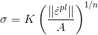
First we load the needed package and define the MFront model. As an example we use the Norton viscoplasticity.
using MFrontInterface, Materials, Plots

norton = raw"""
@DSL Implicit;
@Author Thomas Helfer;
@Date 3 / 08 / 2018;
@Behaviour NortonTest;
@Description {
  "This file implements the Norton law "
  "using the StandardElastoViscoplasticity brick"
}

@ModellingHypotheses{".+"};
@Epsilon 1.e-16;

@Brick StandardElastoViscoPlasticity{
  stress_potential : "Hooke" {young_modulus : 200e3, poisson_ratio : 0.3},
  inelastic_flow : "Norton" {criterion : "Mises", A : 1.0e-5, n : 3.0, K : 100}
};
""";
mfront helper function writes string to file and calls mfront executable to
compile shared library. It also returns the path to the compiled library in tmp folder.
path = mfront(norton)
mat = MFrontMaterialModel(lib_path=path, behaviour_name="NortonTest")
Let's use uniaxial_increment! function from Materials.jl. The first loading
block defines the tension phase and the second the relaxation phase.
s11 = [0.]; e11 = [0.]; tim = [0.]
for i=1:200
dstran = 1e-5
uniaxial_increment!(mat, dstran, 1.0)
update_material!(mat)
push!(e11, mat.drivers.strain[1])
push!(tim, mat.drivers.time)
push!(s11, mat.variables.stress[1])
end
for i=1:500
dstran = 0.0
uniaxial_increment!(mat, dstran, 1.0)
update_material!(mat)
push!(e11, mat.drivers.strain[1])
push!(tim, mat.drivers.time)
push!(s11, mat.variables.stress[1])
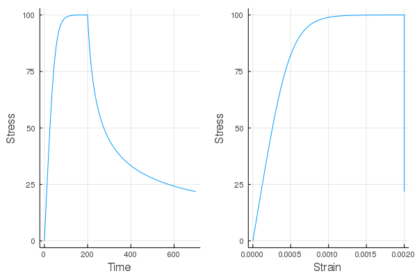
endFinally let's plot the stress-strain behaviour.
p1 = plot(tim,s11,xlabel="Time",ylabel="Stress",legend=false)
p2 = plot(e11,s11,xlabel="Strain",ylabel="Stress",legend=false)
plot(p1, p2, layout=2)
savefig("Norton.png")