ConvergencePlots

This is a Julia package that makes it easy to do live tracking of the convergence of your algorithm. All the plotting is done using PyPlot.jl.

To install ConvergencePlots.jl, run the following Julia code.

using Pkg
pkg"add https://github.com/mohamed82008/ConvergencePlots.jl"

First create an empty plot:

plot = ConvergencePlot()

This will create an empty convergence plot that plots up to 100000 history points. Older points are overwritten. To specify how many history points to plot, use the constructor:

plot = ConvergencePlot(n)

where n is the number of points.

The keyword arguments you can pass to the ConvergencePlot constructor are:

• names: a Vector{String} that has all the names of the convergence metrics to be plotted. The default value of names is ["Residual"].
• options: a dictionary mapping each name in names to a NamedTuple. Each named tuple has the plotting options to pass to PyPlot, e.g. (label = "KKT residual", ls = "--", marker = "+"). If label is not passed, it defaults to the corresponding name in names. You can also pass a single NamedTuple of options without the label option, and it will be used for all the names.
• show: if true the empty figure will be displayed. This is false by default.

After creating an empty plot, you can add points to it as follows:

addpoint!(plot, Dict("Residual" => 1.0))

where the second argument can contain one value for each name in names. If only a single name exists, you can also use:

addpoint!(plot, 1.0)

Adding a point will display the plot by default. To stop the plot from displaying, set the show keyword argument to false.

To close the plot, call:

closeplot!(plot)

using ConvergencePlots

plot = ConvergencePlot(
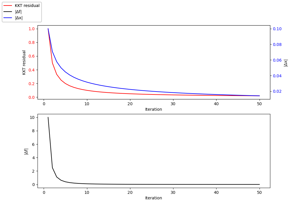
    names = ["KKT residual", "|Δx|", "|Δf|"],
    options = Dict(
        "KKT residual" => (color = "red",),
        "|Δx|" => (color = "blue",),
        "|Δf|" => (color = "black",),
    ),
)
kkt = 1 ./ (1:50)
Δx = 0.1 .* sqrt.(kkt)
Δf = 10 .* kkt .^ 2
for i in 1:50
    sleep(1e-4)
    addpoint!(
        plot,
        Dict(
            "KKT residual" => kkt[i],
            "|Δx|" => Δx[i],
            "|Δf|" => Δf[i],
        ),
    )
end